The first of two Propensity to Cycle Tool (PCT) Advanced Training Workshops took place last week in London, part of the Phase III of the project to inform investments in cycle networks and other interventions for sustainable transport. This post provides an outline of the contents of the workshop, plus links, ideas and sample code. The course was delivered by me (Robin, Lead Developer of the PCT) and my colleague Malcolm Morgan (who led on some of the big data processing and raster tile generation elements of the project). Warning: both of us are heavy R users, so the materials contained plenty of code (more on that soon)!

The good news for people who were unable to attend the first advanced workshop and cannot make the next course in Leeds on the 2^nd August is that all the materials are freely available, following ‘open source’ approach in the PCT: we believe that transport planning should be a more open process. If you already get this, have a good understanding of command line tools for data science and want to crack-on with the content you can do so with reference to the two key materials developed for the workshop:

• The exercises that demonstrate how to get, plot and explore data from the PCT: https://itsleeds.github.io/pct/articles/pct_training.html#exercises
• The slides that accompany the course: https://itsleeds.github.io/TDS/slides/pct-slides.html#1

If you’re interested in attending the next event, you need to complete a form here. On completion, you will be given a link and a password to sign-up. If you’re interested in the wider context, and in attending the next PCT Advanced Training course, read on.

An open source, reproducible approach

The overall aim of the workshop was to get people up-to-speed with the methods and technologies underlying the PCT, to help the design of ‘bikeway networks’ (Buehler and Dill 2016), as part of a wider process of planning for cycle traffic and people, rather than cars (Parkin 2018). The introductory and intermediate training courses used the online interface and the excellent QGIS as the basis for analysing cycle potential. This workshop, however, focussed on working with transport data in R, an open source statistical programming language that can be downloaded from cran.r-project.org and used by anyone for free. The emphasis was on doing interactive data analysis and programming in RStudio, a free and open source integrated development environment (IDE) for R that can be downloaded from rstudio.com.

This ‘command line’ approach allows reproducibility, automation and, once you have overcome R’s steep learning curve, high productivity. Another reason for teaching the Advanced Workshop in R, is that it opens the possibility of extending the PCT, something envisaged in the original PCT paper (Lovelace et al. 2017):

The PCT’s open source license allows others to modify it for their own needs. We encourage practitioners to ‘fork’ the project … and display of the results to suit local contexts. This could, for example, help to visualise city-level targets for the proportion cycling by a certain year and which will vary considerably from place to place in ways not yet well understood. Modifying the code base would also allow transport planners to decide on and create the precise set of online tools that are most useful for their work.

The PCT R package

An important aspect of the PCT, which we advocate others developing publicly funding transport modelling tools to adopt, is that it is open source and based on open data, ensuring transparency, reproducibility, and preventing monopolisation by single companies and ‘cloud lock-in’. These are vital if transport modelling is to be a fully fledged part of an open and democratically accountable transport planning system, that is part of the democratic process.

‘Open source’ means you can see the PCT’s codebase, which is hosted at github.com/npct. Rather than use this codebase, which was developed using R packages such as sp that are now slightly out of date, we taught the course based on data that could be downloaded in the sf class system (if that sounds like double Dutch to you, see an explanation here). Data was provided by pct, a small R package that was written to enable ease of access to data and methods underlying the PCT from R’s command line interface. For more on the package, the latest version of which has just been released on CRAN, see it’s online home at itsleeds.github.io/pct.

In terms of learning objectives, the aim was for participants able to be able to do the following things, with help from the **pct* R package:

• Understand the data and code underlying the PCT
• Download data from the PCT at various geographic levels
• Use R as a tool for transport data analysis and cycle network planning

The workshop was divided into two halves. Before lunch, we provided an overview of the PCT project with a focus on the different types of data used in the PCT and some of the strengths, limitations and opportunities of the national PCT data, with reference to an academic paper that provides an overview of the approach Lovelace et al. (2017). After lunch, we progressed to a ‘minihack’ during which participants were provided with an opportunity to apply the methods to their own data.

Datasets processed

In terms of the input data, the concept of a ‘data hierarchy’ was used to introduce the various geographic levels of the data used in the PCT, with reference to Chapter 6 (Transportation) of the open source and publicly available book, Geocomputation with R (Lovelace, Nowosad, and Meunchow 2019). At the base of the pyramid is zonal data, which is widely available yet highly aggregated. In the PCT, zones represent, on average, around 6000 people (around half of whom commute) at the Middle Super Output Area (MSOA) level, and around 1200 people at the Lower Super Output Area (LSOA) level. The key data level used by the PCT, however, is origin-destination data, which forms the basis of the route and route network levels. These datasets are generated using the following processes:

• Origin-destination (OD) data processed using functions such as od2line() in the stplanr R package (Lovelace and Ellison 2018)
• Route network generation and analysis
• Route allocation using different routing services
• Geographic desire lines

These stages were illustrated in the Isle of Wight, a relatively small and self-contained region that is ideal for testing. The starting code to analyse car-dependent routes on the island was as follows:

library(sf)
library(pct)
library(dplyr) # suggestion: use library(tidyverse)
z_original = get_pct_zones("isle-of-wight")
z = z_original %>% 
  select(geo_code, geo_name, all, bicycle, car_driver)
l = get_pct_lines("isle-of-wight")
plot(z$geometry)
lwd = l$all / mean(l$all)
plot(l["bicycle"], lwd = lwd, add = TRUE)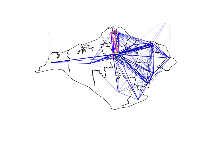

We rapidly progressed through the course, to analyse cycling potential at route and route network levels, using a small input dataset representing 30 key desire lines on the Isle of Wight. Exercise for the reader: see if you can run the code chunk below (after running the previous chunk), to generate this plot:

library(tmap)
library(stplanr)
tmap_mode("view")
route_data = st_sf(st_drop_geometry(wight_lines_30), geometry = wight_routes_30$geometry)
rnet = overline2(route_data, "dutch_slc")
tm_shape(rnet) +
  tm_lines(lwd = "dutch_slc", col = "blue", scale = 7) +
  tm_shape(route_data) +
  tm_lines(col = "bicycle", lwd = "all")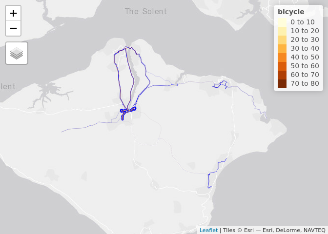

Next steps

Rather than explain what is going on here, this post (nearly) finishes by guiding readers towards further resources on the study of cycling potential at the command line:

• Paper on the stplanr paper for transport planning (available online) (Lovelace and Ellison 2018)
• Introductory and advanced content on geographic data in R, especially the transport chapter (available free online) (Lovelace, Nowosad, and Meunchow 2019)
• Paper on analysing OSM data in Python (Boeing 2017) (available online)

Next course

The final thing to say is that there is another PCT Advanced Workshop upcoming, this time in Leeds, on the 2^nd August. If you would like to attend, please check out the course prerequisites, complete the test code (which you can find here) and, if you think it’s right for you, complete the form here. On completion, you will be given a link and a password to sign-up.

References

Boeing, Geoff. 2017. “OSMnx: New Methods for Acquiring, Constructing, Analyzing, and Visualizing Complex Street Networks.” Computers, Environment and Urban Systems 65 (September): 126–39. https://doi.org/10.1016/j.compenvurbsys.2017.05.004.
Buehler, Ralph, and Jennifer Dill. 2016. “Bikeway Networks: A Review of Effects on Cycling.” Transport Reviews 36 (1): 9–27. https://doi.org/10.1080/01441647.2015.1069908.
Lovelace, Robin, and Richard Ellison. 2018. “Stplanr: A Package for Transport Planning.” The R Journal 10 (2): 7–23. https://doi.org/10.32614/RJ-2018-053.
Lovelace, Robin, Anna Goodman, Rachel Aldred, Nikolai Berkoff, Ali Abbas, and James Woodcock. 2017. “The Propensity to Cycle Tool: An Open Source Online System for Sustainable Transport Planning.” Journal of Transport and Land Use 10 (1). https://doi.org/10.5198/jtlu.2016.862.
Lovelace, Robin, Jakub Nowosad, and Jannes Meunchow. 2019. Geocomputation with R. CRC Press. http://robinlovelace.net/geocompr.
Parkin, John. 2018. Designing for Cycle Traffic: International Principles and Practice. ICE Publishing. https://www.icevirtuallibrary.com/isbn/9780727763495.
Reblogged this on Geosaber.